Modeling disk galaxy rotation curves with MaNGA and Stan

• by mlpeck

  I'm giving away ideas. Code too, if anyone wants it. Stan by the way is a probabilistic modeling language. The name is not an acronym.

  I've been studying MaNGA data off and on since the first public release a little over a year ago. One of the things you need to do anything else with the data is a set of redshift or velocity offsets, and since the MaNGA team hasn't yet published their own measurements I developed my own routine for that task. I've thought a little bit about how to get rotation curves out of the measured velocity fields but wasn't quite getting to a solution. There's lots of literature out there but some of the methods used seem pretty dodgy and specific implementations are written in languages like IDL and Fortran. No thanks.

  But a few weeks ago a paper showed up on arxiv by Oh et al. 2017: "2D Bayesian automated tilted-ring fitting of disk galaxies in large HI galaxy surveys: 2DBAT." I liked the idea of what they're doing, but I didn't care much for the implementation so I decided to try my own (slightly simplified) version in Stan, which I've been using for a few years now. After a couple false starts and some discussion on the Stan help forum I got a workable model. Here are some early results.

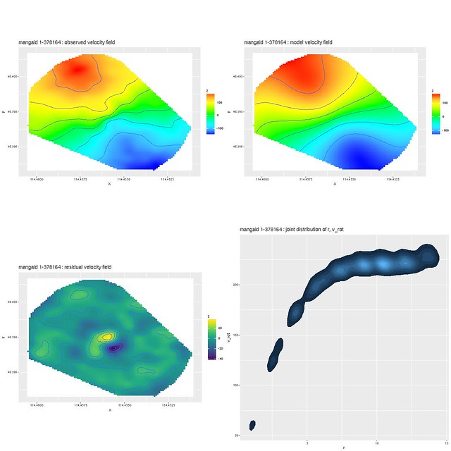
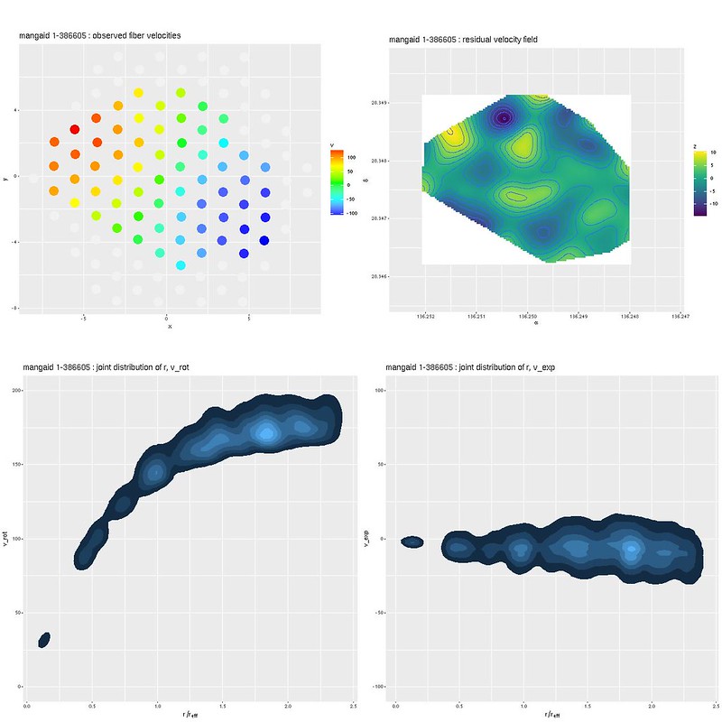
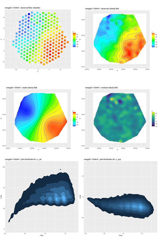
  First is one of the Masters et al. red spirals:

  

  Here are some select model results. These show the measured and model velocity field, the residuals from the model, and the derived rotation curve. The latter is shown as the joint density of the deprojected radius in arcseconds and the rotational velocity. There's interesting deviations from the model on either side of the nucleus and it looks like there are departures from circular motions in the arms as well.

  

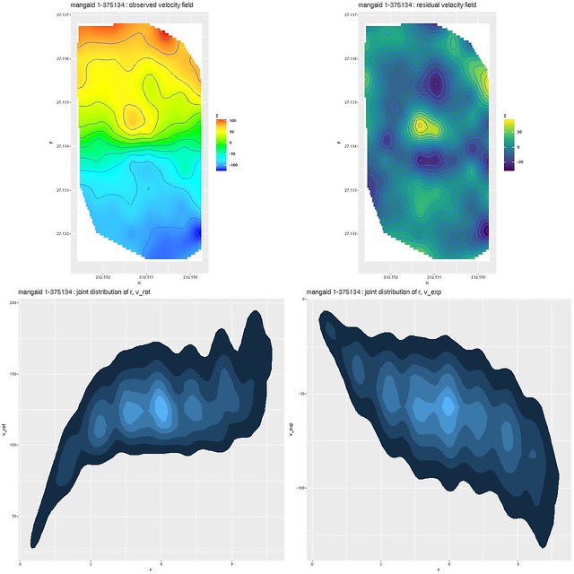
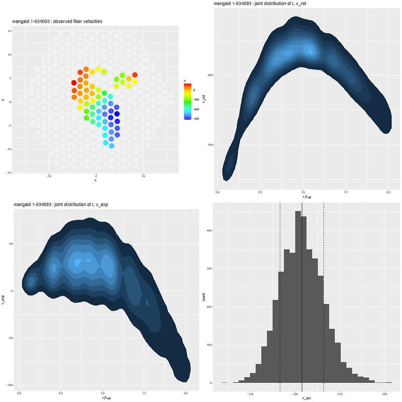
  Here's another one that's a little more peculiar. This came from one of the truly passively evolving spirals that I've tentatively identified.

  

  This one shows some an interesting sinusoidal pattern of residuals from the model velocity field along or maybe offset a little bit from the bar. This model also estimates two components of velocity. One, labeled v_exp in the plot below is I think meant to estimate radial streaming motions. That should be small but in this run it's quite large and varies significantly with radius. I'm not sure what the significance of any of this is.

  

  So far just about all the examples I've looked at have rising velocity curves out to the edge of the collected data. That's not too surprising because the MaNGA spectroscopy isn't very deep. Unfortunately there isn't any literature yet to compare my results to.

  Later perhaps I may follow up with more examples and more in depth discussion of the models, when and why they fail, and how to distinguish bad model runs from good.

  Posted October 2, 2017 5:29 PM

• by mlpeck

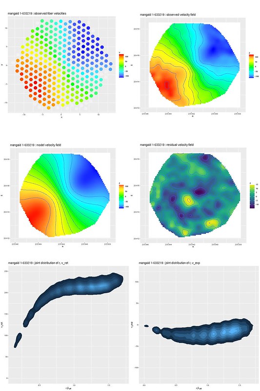
  One more from the Masters et al. red spiral sample. Finder chart:

  

  Measured and model velocity fields, model rotation and radial velocity vs. deprojected radius:

  

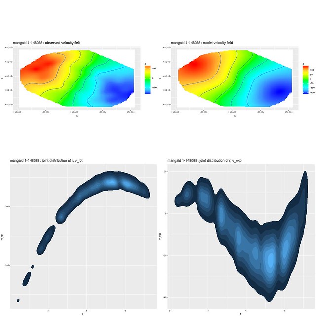
  By the way the model I implemented is a fairly standard "tilted ring" representation that decomposes the radial velocity field into orthogonal components that are supposed to represent circular and radial (within the disk) components. A large radial component as in the example in the previous post (and maybe here too) probably indicates model misspecification. Spekkens & Sellwood (2007) fomulated a similar looking model with different symmetry to represent bar distortions.

  I plan to look at that model formulation too, but I probably won't have time before I have to go do something else.

  Posted October 4, 2017 4:55 PM

• by mlpeck

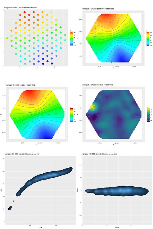
  One more before I'm outta here for a while. This is UGC 9105, a non-barred spiral from the Masters et al. blue sample.

  

  Again, measured and model velocity field, circular velocity and radial (in the disk) velocity vs. deprojected radius (in arcseconds):

  

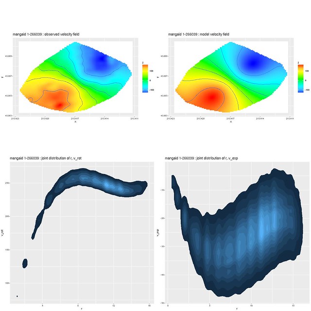
  This looks like a really good fit with no systematic departures from the model velocity field. There are still significant non-circular motions though.

  By the way this short review of the structure and dynamics of the inner Milky Way gives some helpful context. The sun's rotation velocity is estimated to be 238 km/sec. and it's located a little more than 8 kpc. from the center. That would put it at about 11.5" on this graph or at about 7" on the one I posted yesterday. The milky way's rotation curve looks a bit like this one but with a faster initial rise. Morphologically it's probably more similar to the barred spiral I posted yesterday though.

  Posted October 5, 2017 5:01 PM

• by JeanTate

  Very cool results, mlpeck! 😃

  I'm having difficulty, however, in reading the "joint distribution ..." plots; for example I can't work out what the axes (both x and y) are, nor the values of the tick marks. Can you clarify please?

  Also, where did you get the value of the inclination parameter from, to do the deprojection?

  Oh, and only one of the galaxies looks like "red spiral", unless they are being classified by their apparent color of only the inner parts (the outer parts of all appear very much "blue" in all but 1-175134).

  Posted October 5, 2017 6:09 PM

• by mlpeck

  Hi Jean:

  Sorry, those plots got compressed to illegibility to fit in the space Talk allows. Full resolution versions are on my Flickr page at https://www.flickr.com/photos/27794530@N08/. The 4 most recently posted (as of 5 October) are the ones in this series of posts.

  The x axis in the joint distribution plots is deprojected radius in arcseconds. The y axis is velocity in km/sec. Scales vary. Better units for radii would be kpc or relative to the effective radius. Maybe when I have time to work on this again.

  I guess the inclination parameter. The guess is used both to initialize the parameter for sampling and also to set the prior, and then I hope the data actually has something to say about the real inclination. I'm pretty sure the SDSS photometric pipeline produces quantities that would allow more refined guessing. This is a huge source of potential error (both random and systematic) by the way. The inclination angle and rotation speed are, as astronomers like to say, highly degenerate.

  You'd need to reconsult the original Masters et al. paper for their selection criteria, but it was based on galaxy-wide color measurements (I forget which one). It's fairly obvious just browsing thumbnails of the whole sample that the red spirals really are redder than blue ones overall. Of course it's also obvious that just about all of them have evident H II regions in their disks.

  The galaxy with mangaid 1-375134 is not in the Masters et al. sample. It was one of a smallish number of spirals in MaNGA that I identified with a casual search as possible candidate truly passively evolving galaxies. It's quite odd looking, no? I think it's a lenticular in the making, or perhaps evolving into a rotating spheroid.

  Posted October 5, 2017 10:14 PM

• by JeanTate in response to mlpeck's comment.

  Thanks Mike.

  The x axis in the joint distribution plots is deprojected radius in arcseconds.

  As they all start at (near) 0, I'm guessing you've assumed symmetry, and "summed" (in some way) azimuthally (?), centered on the galaxy's photocenter (or what the model found as the nucleus?). Am I close?

  I guess the inclination parameter.

  FWIW, I think the textbook approach is to assume a flat, symmetric disk; the observed minor/major axis ratio can then be used to estimate the inclination. Traditionally, I think the idea was to take the outermost isophote ("B25") as defining the "edge" of the disk.

  I'm pretty sure the SDSS photometric pipeline produces quantities that would allow more refined guessing.

  Yes, PhotoObj has two sets of parameters that are relevant, deVAB and ExpAB (one for each band), the fit for an ellipse assuming an otherwise symmetric deVaucouleurs (Sérsic index 4) and an exponential intensity profile (Sérsic index 1), respectively.

  Of course, even if in an isolated environment, evolving in a purely secular way, real spiral galaxies may not be nice, flat, symmetric disks! So if a model assumes that, it may produce somewhat unrealistic results.

  Of course it's also obvious that just about all of them have evident H II regions in their disks.

  Which raises an interesting question: does the observed motion of the gas (plasma) faithfully reflect the motion of the stars? If I recall correctly, in nice and (apparently) stable spirals (other than Sdm, and Sm types perhaps), the stellar mass is dominated by relatively low-mass main sequence stars, whose motion is totally dominated by gravity. However, for galaxies with lots of star-formation, the ISM which emits the H-alpha (etc) is influenced by shock fronts, collisions, and (maybe) magnetic fields. No doubt some of this motion will have an out-of-plane component (i.e. orthogonal to the disk); I don't know to what extent your v_exp can distinguish between this motion and in-disk streaming.

  It's quite odd looking, no? I think it's a lenticular in the making, or perhaps evolving into a rotating spheroid.

  I'd say it's unusual, a truly red, bar-dominated, tiny nucleus, two-arm spiral. I've been reading up on lenticulars (S0 galaxies), and there's several papers (by big names!) presenting a case that the S0s are a parallel sequence, to the spirals, and thus likely formed by different mechanisms (and over different timescales).

  Posted October 8, 2017 9:28 PM

• by mlpeck in response to JeanTate's comment.

  As they all start at (near) 0, I'm guessing you've assumed symmetry,
  and "summed" (in some way) azimuthally (?), centered on the galaxy's
  photocenter (or what the model found as the nucleus?). Am I close?

  The model assumes strict axisymmetry and decomposes the measured velocity into two components each of which is a function of radius only. One is circular and the other is interpreted as "expansion" velocity. This is pretty standard -- this is the model outlined in the arxiv paper I linked in the OP (equations 1-5 iirc) or for example in this review by Teuben (2002). There is also a residual term that accommodates some degree of model misspecification.

  As I mentioned in an earlier post there are alternative formulations that may, for example, be more appropriate for barred galaxies. The general formulation of tilted disk models also allow for varying inclination and orientation of the "rings." I don't think it's going to be productive to allow varying inclination with MaNGA data. For one thing the spectroscopy isn't very deep and warps aren't likely to be common in inner disks of apparently undisturbed galaxies. Varying inclination is something I'll look at. It's generally best to start simple with models like this and add complications later as data demands (or allows).

  Which raises an interesting question: does the observed motion of the
  gas (plasma) faithfully reflect the motion of the stars? If I recall
  correctly, in nice and (apparently) stable spirals (other than Sdm,
  and Sm types perhaps), the stellar mass is dominated by relatively
  low-mass main sequence stars, whose motion is totally dominated by
  gravity. However, for galaxies with lots of star-formation, the ISM
  which emits the H-alpha (etc) is influenced by shock fronts,
  collisions, and (maybe)

  The MaNGA DRP calculates separate velocity fields for ionized gas and stars, but so far I only return a single value that could be dominated by either. From what I've seen of their sample data sets usually one or the other is of considerably lower quality and a "blended" estimate is likely to be better. On the other hand if stars and gas aren't tightly coupled my method fails. The one Manga paper I remember seeing that was primarily about kinematics was about decoupled gas and stars, which happens in a not entirely trivial minority of galaxies.

  I managed to get my Stan code and a sample data set uploaded to github before I had to put this project away for a while: https://github.com/mlpeck/vlos_stanmodels. It's really amazing how little code is needed to express a complete model.

  Posted October 9, 2017 4:14 PM

• by klmasters scientist, admin

  Beautiful stuff Mike. 😃

  Posted October 19, 2017 4:17 PM

• by zookeeper admin, scientist

  This is great! Would you like to write this up? I'd be happy to help, and I think astronomers would be interested.

  Posted October 20, 2017 8:54 AM

• by mlpeck in response to zookeeper's comment.

  Yes, I'd be interested. You should find a student in need of a project though! There are legitimate research opportunities I think in addition to the possibility to learn some new techniques.

  Posted October 20, 2017 5:47 PM

• by mlpeck

  Month later update: @zookeeper (Chris Lintott I assume) suggested writing something up, but there hasn't been any followup on what to write up. A writeup could be anything from a short tutorial case study to a techniques paper intended for publication to a full blown research project. The only issue I'd have with a techniques paper is that for techniques that are new to the intended audience it's pretty much de rigeur to apply your technique to fake data, and that's something I find boring. I prefer to dive right in to real data and see if I can make any sense out of it.

  Yes, PhotoObj has two sets of parameters that are relevant, deVAB and
  ExpAB (one for each band), the fit for an ellipse assuming an
  otherwise symmetric deVaucouleurs (Sérsic index 4) and an exponential
  intensity profile (Sérsic index 1), respectively.

  Jean, the MaNGA targeting catalog (in a table named mangadrpall in CASJOBS, or separately downloadable from SAS) has quite a lot of metadata from the Nasa-Sloan Atlas, which was developed to rectify some of the problems with SDSS photometry of larger galaxies that I know you're quite familiar with. A couple of those are useful for sample selection and model initialization; there are two estimates of the major axis angle and two of the ratio of minor to major axis diameters. The ones that are recommended to use are "elliptical petrosian" estimates. Those are "nsa_elpetro_phi" and "nsa_elpetro_ba" respectively. Also in the table are "nsa_elpetro_th50_r" which is the recommended estimate of effective radius, and "nsa_sersic_n" which is the sersic index of single component sersic fits to the photometry (I think r band is reported).

  I've been working at a leisurely pace on three things:

  1. Selecting a sample of (probable) disk galaxies.
  2. Batch processing -- can the modeling be automated?
  3. For a first look I just used low order polynomials to characterize the circular and "expansion" velocity components. I'd like a more flexible representation. Spline basis functions are the obvious choice, but I haven't gotten that to work yet. I'm still hopeful.

  Posted November 19, 2017 6:01 PM

• by mlpeck

  So, how are action items 1-2 going?

  I had a couple preliminary ideas about sample selection. One idea is just to use a known sample of disk galaxies and an obvious choice for that would be the combined Masters et al. blue+red spiral sample. There are 69 total of those in the second MaNGA release based on position cross match. This is truly a pure spiral sample with no obvious false positives, but it is by design also incomplete. I'll probably end up looking at it anyway.

  My other preliminary thought was to try to select a sample with a query of the drpall table. Some paper I looked at recently used a sersic index < 2.5 to select disk galaxies -- sorry, I don't have a cite for this at the moment. Inclination angles between about 20 and 70 degrees are considered suitable candidates for tilted ring analysis. I decided to be more conservative and select objects with estimated inclination angles between 30 and 60 degrees. For a true circular disk the minor to major axis ratio estimates the cosine of the inclination, so this selection criterion is 0.5 ≤ nsa_elpetro_ba ≤ 0.866.

  MaNGA has two main samples: the primary sample is observed to a length scale of about 1.5 effective radii. There's also a secondary sample observed to a length scale of 2.5 effective radii. The visible extent of primary sample galaxies is considerably larger than the IFU (the ones I posted about earlier are all from the primary sample). Secondary sample galaxies have pretty much their full visible extent in SDSS imaging covered by the IFUs. Hoping to get measurements as far out in disks as possible I decided to first look at secondary sample galaxies, which are identified with the targeting bitflag 2048 ≤ mngtarg1 < 4096. Those three criteria produce a sample of about 350 250 galaxies.

  In thumbing through the sample I noticed several problems with my reasoning. Most importantly, although the spatial coverage is greater the spectroscopy isn't any deeper than the primary sample so the fraction of usable data for any given object is typically quite low. Some related problems are that in order to get a large enough sample that fits within the available IFU sizes they had to extend the candidate sample to fairly high redshifts and therefore the typical redshift of a secondary sample galaxy is higher than a typical primary sample galaxy. That means the spatial resolution is typically lower. There also seems to be a preponderance of rather low surface brightness objects in the secondary sample. I don't know if that's due to cosmological effects or some other peculiarity of the sample selection algorithm but it further reduces the amount of data suitable for analysis.

  Can modeling be automated? Yes it can, with some caveats.

  Posted November 19, 2017 7:15 PM

• by mlpeck

  Can modeling be automated? Yes it can, with some caveats.

  A couple preliminaries. There are two angles (or more generally sets of angles) involved in a tilted disk model of rotation curves. One is an orientation that is conventionally defined as the angle measured counterclockwise from north to the direction of the major axis. The other is the tilt or inclination of the disk, with face on defined to be 0°.

  In any data analysis it's important to distinguish between data and model parameters. Data is, well, data. It's what you've measured. Parameters are the things whose values you're trying to estimate. I mentioned two posts up that estimates of both the orientation angle and inclination are provided in the MaNGA targeting catalog. So are these parameters or data? In the context of kinematic modeling they could be either, but I treat them as model parameters; that is I'm hoping the data will tell me something about their values. There are two basic reasons for this:

  1. The estimates provided are from the photometry. We're interested in kinematic quantities, which aren't necessarily the same.
  2. Treating angles as data with fixed values will lead to severely underestimating the uncertainty in the rotational velocity curve. This is especially the case with the inclination angle, which is nearly degenerate with circular velocity (that is, in a Bayesian context the posteriors are highly correlated).

  I use the catalog values for two purposes. First, any nonlinear optimization or MCMC simulation requires a set of starting values for parameters. For automated processing the catalog entries provide suitable starting guesses. This is more important for the orientation angle. A generic guess of 45° for the tilt might work as well or even better in some cases.

  The second use for them is to set the priors. I set the central value for the orientation's prior to the catalog value. I've experimented with using either the catalog ba value or a generic guess of 45° for the central value of the prior for tilt. For technical reasons that I'll save for a more formal writeup it's necessary to make the priors at least somewhat informative. I use generic values for the widths (that is, standard deviation) of the priors.

  There are several other parameters in the model including the position of the kinematic center measured as offsets in x and y coordinates from the IFU center, and an overall systemic velocity. These should all be small. Except for a few cases in early commissioning observations the IFU is almost always centered close to the photometric center, which in turn should be close to the kinematic center for an undisturbed disk. I measure the velocity field as offsets from the system redshift, which is usually quite accurate and close to the central velocity. The priors for these quantities are therefore centered on 0 with generous, but finite, widths.

  In the current version of the models the remaining parameters are the coefficients of the terms of the polynomials describing the circular and "expansion" velocity. Except for the linear term of the circular velocity these should be fairly small with either sign. I give them generic broad (but again, proper) priors.

  First caveat: the photometric orientation angle is only determined modulo π while the kinematic angle is determined modulo 2π -- by convention the angle is measured to the receding side. For early experiments I just plotted the velocity field and eyeballed the angle. Technically this is cheating I think, but experts on Bayesian modeling don't seem too concerned. For automated processing it actually doesn't matter if the orientation is off by 180°, because the sign of the circular velocity will just flip.

  Later, more caveats including problems that can crop up with blind sample selection and specific issues with my initial sample...

  Posted November 22, 2017 4:35 PM

• by mlpeck

  Two posts up I talked about some possibilities for sample selection, and mentioned one selection of ∼250 probable disk galaxies from the "secondary" MaNGA sample. Here are a couple examples. First is one that worked out really well -- here is an SDSS postage stamp with the IFU outline overlaid:

  

  Here are selected results from rotation curve modeling. The upper left pane is the measured velocity field. I use, by the way, the "row stacked spectrum" (RSS) files not the data cubes. There are reasons for that. I haven't figured out how to do Voronoi binning yet and binning is probably not appropriate for kinematic modeling anyway. Instead I select a very optimistic S/N threshold and analyze the spectra that pass it. In this case I was able to use a little over half of the spectra, and the velocity field clearly indicates rotation.

  The circular velocity curve in the lower left pane looks reasonable. The model I implemented decomposes the measured velocity into rotational and radial components (usually referred to as "expansion"). Both are treated as being strictly axisymmetric. The expansion velocity should be small if stars and gas are really on circular orbits and in this case it is as indicated in the lower right pane. And, the fit to the data is good as seen in the upper right. This is about as good as it gets.

  

  This next one illustrates several problems. First of course there are clearly (at least) two galaxies here. Are they interacting or just an accidental overlap? I'd say interacting, but for modeling purposes it sorta doesn't matter because my redshift measurement routine only returns one value and there's no way to control which value will be returned from blended spectra. This sample is small enough to be easily looked through using the SDSS image list tool and this one should probably have been rejected, but it slipped into my initial list of candidates for batch processing anyway.

  Another problem is, as I guessed, even though the IFU covers the whole visible extent of the galaxy the exposures aren't any deeper so the fraction of usable data is very low -- only about 16% in this case.

  

  Well, the velocity field (top left below) is pretty neat. I got measurements for the disk and some ways out in the spiral arms of the larger galaxy, and several fibers covering the smaller one. Stan happily cranks out a model for this, but the rotation curve is almost certainly spurious.

  One thing it did get right is the system velocity of the larger galaxy. The SDSS spectrum for this pair was centered on the smaller galaxy, and that's what was used for the system redshift in the NSA atlas. It turns out the larger galaxy is blueshifted a little bit relative to the smaller one, by -118±5 km/sec as indicated in the lower right pane.

  

  Next up, when I get around to it, some results from the Masters et al. spiral sample and maybe some musing about further ideas for sample selection.

  Posted November 29, 2017 5:31 PM

• by mlpeck

  One more post and I'm outta here again for a while. I modeled the Masters et al. spiral sample. By my count there are 68 unique galaxies in the first two MaNGA public releases, with 65 from the "blue" spiral sample and 3 from the reds. It actually turns out to be easy to automate the modeling. Neither the velocity field measurements nor the rotation curve modeling require manual intervention. There were about a dozen galaxies where the velocity fields were corrupted by foreground stars or galaxy overlaps. It wouldn't be too hard to mask the bad data by hand, but I haven't done it.

  The main problem with the Masters sample is it was selected to be close to face on, and they were highly successful at that. There are at least 10-12 galaxies in this sample with inclinations under 20 degrees, which is a pretty optimistic limit for successful rotation curve modeling.

  Here are three examples of model runs (higher resolution copies are on my flickr page). I show the same data for each galaxy. First are the actual measured velocity offsets. The symbols aren't quite the size of the fibers, which almost fill the IFU area. I used a "thin plate spline" routine for interpolating spatial data and that was used to produce the next three plots, which are the velocity field again, the model velocity field, and residuals (difference between the observed data and models). Next are modeled circular and "expansion" velocities plotted against radius in units of the cataloged effective radius.

  The first two appear to be good models. The third is right at the limit of being usable because of low inclination. Notice the posterior uncertainty in the circular velocities are very large, as they should be.

  

  

  

  Here are finder chart images for these three:

  
  
  

  Posted December 1, 2017 10:03 PM

• by mlpeck

  I haven't posted in a while, but I have been working on this as time permits. I've made significant updates to my github project page at https://github.com/mlpeck/vlos_stanmodels. There is an additional Stan model there, R code that should if I didn't forget anything make it possible to recreate my workflow starting from any MaNGA RSS file, and some supplemental data sets in R binary format that are needed in analyses. There's also a README with some instructions and a link to a sample data file. Although I haven't used them in kinematics models there's also code to read the data cube fits files and store them in a format suitable for further analysis.

  One of these days I will try to write up some sort of tutorial case study. There are two potential audiences for that, so it may be worth the effort even though this is just a hobby for me.

  One of these days I'll try to do a Python port. For the most part it shouldn't be difficult except I find it hard to jump back and forth between R and Python and I need to spend some time refreshing my Python skills (and staying away from R while doing it).

  Posted January 25, 2018 5:31 PM